
In my previous post Road testing kallisto, I presented the results of a simulation study to test the accuracy of kallisto. Specifically, I hypothesised that kallisto would perform poorly for transcripts with little or no unique sequence and I wanted to use the simulation to flag these transcripts in my downstream analysis. The simulation was therefore intentionally naive and ignored biases from library preparation and sequencing so I could focus on the accuracy of quantification with “near perfect” sequence reads. The simulation results broadly fitted my expectations but also threw up a few more questions in the comments section. I’m going to post an update for each of the following questions:
- What’s the impact of including low-support transcripts on the quantification of well-supported transcripts?
- The correlation between truth and estimated counts drops off as a transcript has fewer unique k-mers. Is this also reflected in the bootstrap variances?
- How does kallisto compare to sailfish, salmon and cufflinks?
- This comparison will come with caveats because of the way the reads were simulated
For this post I’ll focus on the first question.
The impact of including low-support transcripts on the quantification of well-supported transcripts
Previously I showed that the 9 DAZ2 transcripts (Ensembl v82) are very poorly quantified by kallisto. DAZ genes contain variable numbers of a repeated 72-bp exon (DAZ repeats) and I noted that transcript models for DAZ2 overlapped one another perfectly with regards to the splice sites, so some isoforms differ only in the number of DAZ repeats, hence 8/9 of the isoforms had no unique kmers whatsoever. I further suggested that the inclusion of low-support transcript models in the gene set may be reducing the accuracy of quantification for the high-support transcripts. I then suggested this was likely to be a problem at many other loci and filtering out low-support transcripts may be beneficial.
To test this, I created two genesets, “Filtered” and “Unfiltered“, both containing transcripts from hg38 Ensembl v82 protein-coding genes. For the “Filtered” gene set I removed all transcripts with a low-support level (>3 ; No supporting non-suspect EST or mRNA). For the “Unfiltered” gene set, I retained all transcripts. I then compared the accuracy of quantification over all transcripts with a support level of 1-3.
We would expect this filtering to increase the fraction of unique 31-mers in the remaining transcripts. Figure 1 demonstrates that this is indeed the case.

Figure 1. Distribution of fraction of unique 31-mers per transcript in the filtered and unfiltered gene sets
Figure 2 is a re-representation of the the previous figure showing the correlation between the sum of ground truths across the 30 simulations and the sum of estimated counts, with separate panels for the two gene sets. The two panels only show quantification over the high-support transcripts. There’s a clear but slight decrease in the accuracy of quantification when using the unfiltered gene set. With the arbitrary threshold of 1.5-fold that I used previously, 278 / 97375 (0.28%) are flagged as “poor” accuracy, compared to 448 / 97375 (0.46%) when we include the low-support transcripts. Honestly, I was expecting a bigger change but this hard thresholding somewhat masks the overall decrease in accuracy.

Figure.2 Filtering low-support transcripts improves the quantification accuracy for high-support transcripts with kallisto
Figure 3 shows the same plot but focusing on the DAZ genes. All the transcript models for DAZ4 are support level 5 so this gene is not included. When the gene set is not filtered, one of the DAZ1 (ENSG00000188120) transcripts is accurately quantified, with the other transcripts having zero or close-to-zero estimated counts across the 30 simulations. The filtering leads to a much improved quantification accuracy for the other DAZ1 transcript and one of the DAZ2 (ENSG00000205944) transcripts. However, there is no real improvement for the remaining transcripts, with two now considerably over-estimated and the other 4 showing no improvement.
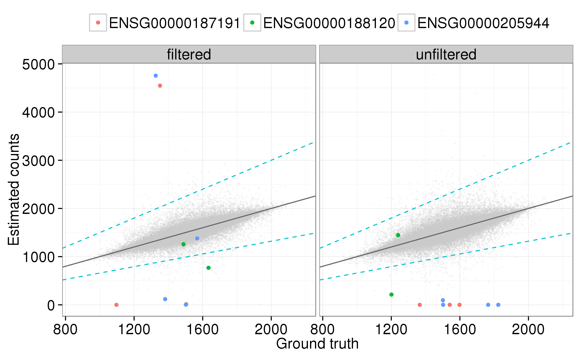
Figure 3. Improvement in quantification of DAZ gene transcripts when low-support transcripts are filtered out
The other important metric when assessing the accuracy of quantification is the Pearson’s correlation coefficient (r) between the ground truth and estimate counts across the simulations. For the majority of transcripts r>0.9 even when using the unfiltered gene set, however there is a noticeable improvement when the gene set is filtered (Figure 4).

Figure 4. Distribution of Pearson’s correlation coefficients between ground truths and kallisto estimated counts across 30 simulations. Transcripts were quantified using a filtered and unfiltered gene set
We would expect the greatest improvement where the correlation is low with the unfiltered gene set and the filtering leads to a large gain in the fraction of unique 31-mers. To show this, Figure 5 presents the gain in fraction of unqiue 31-mers (x-axis) against the improvement in correlation with the filtered geneset (y-axis), split by the correlation when using the unfiltered geneset. The transcripts in the top left panel showed very poor correlation with the unfiltered gene set (<0.5), so improvements here may be partly affected by regression to the mean. Looking at the other panels which show the transcripts with correlation >0.5 when using the unfiltered gene set, we can see that as the gain in fraction of unique 31-mers approaches 1 the improvement in the correlation tends towards the maximum possible improvement. Even those transcripts which only show a very slight gain in the fraction of unique 31-mers show a considerable improvement in the correlation. This is in line with my observation in the previous post that kallisto shows a much better performance for transcripts with > 0.05 unique kmers. 11047 / 97375 (11.3%) of high-support transcripts show at least a 0.05 increase in the fraction of unique kmers.

Figure 5. Change in correlation when using the filtered gene set relative to the unfiltered gene set, split by the gain in fraction of unique 31-kmers and the correlation in the unfiltered gene set
Summary
The figures I’ve shown here fit perfectly with the expectation that filtering out the low-support transcripts increases the fraction of unique kmers in a subset of the remaining transcripts, in turn improving the accuracy of the estimated counts from kallisto. Removing the 44023 low-support transcripts improves the accuracy of the sum of estimates for the high-support transcripts, but the improvement is only slight. Whether this gain is worth removing 44023 isoforms is really down to how much you believe these low-support isoforms. Personally, I worry that a lot of these low-support transcripts are spurious models from poor transcript assembly.
The DAZ genes provide an insight into a very hard-to-quantify set of transcripts, indicating that there are gains to be made from filtering out the low-support transcripts but in some instances these will be minimal. Indeed, in some cases, even transcripts we know are real are just going to be near-impossible to quantify with short-read RNA-Seq due to their sequence similarity with other transcripts from the same locus and/or homologous loci.
The improvement to the correlation across the 30 simulations is somewhat clearer than the improvement in the sum of estimates, and most prominent where the gain in unique kmers is greatest, as expected. 11.2% of transcripts show a significant improvement in the fraction of kmers which seems to me a worthwhile gain for the loss of the low-support transcripts from the gene set. The next step will be to explore the effect of the filtering on differential expression analysis, since this is what I want to use kallisto for, and I expect this will be it’s major use case.
UPDATE (22/10/15):
In response to Ian’s question below, I had a look at whether removing a random selection of transcript models has a similar impact on the accuracy of the remaining models. To do this, I identified the number of transcripts which would be removed by the transcript support level (TSL) filtering for each gene_id and removed a random set (of the same size) of transcript models for the gene_id. This should ensure the comparison is “fair” with regards to the complexity of the loci at which transcript models are removed and the total number of transcript models filtered out.
My expectation was that low-support transcripts would be contaminated by transcript models from incomplete transcript assembly and would therefore be shorter and show a greater overlap with other transcript models from the same locus. I therefore expected that the removal of the random transcripts would also increase the fraction of unique kmers, as suggested by Ian, but that the effect would be greater when the low-support transcripts were removed. It turns out I was wrong! Figure 6 shows the distribution of fraction unique 31-mers with the unfiltered, TSL-filtered and randomly filtered annotations. The random filtering actually leads to a slightly greater increase in the fraction unqiue 31-mers for the remaining transcripts. This also leads to an slightly greater correlation for the remaining transcripts (Figure 7).
So what about the length and overlap of the low support transcripts? Well it turns out the transcript models do decrease in length from TSL1-4, but oddly transcripts with TSL 5 (“no single transcript supports the model structure”) are very similar in length to TSL1 transcripts (Figure 8). To compare the overlap between the transcript models, I took a short cut and just used the fraction unique kmers as a proxy. Transcripts which have more overlap with other transcripts from the same locus will have a lower fraction of unique kmers. This is complicated by homology between gene loci but good enough for a quick check I think. Figure 9 shows the fraction unique kmers at each TSL. Again TSL1-4 show a trend with TSL5 looking more similar to TSL1 & 2. Interestingly the trend is actually in the opposite direction to what I had expected, although this comes with the caveat that I’m not controlling for any differences in the genome-wide distribution of the different TSLs so I’d take this with a pinch of salt.
Why TSL5 transcripts are more similar to TSL1-2 transcripts I’m not sure, perhaps this scale shouldn’t be considered as ordinal after-all. I think I’d better get in contact with Ensembl for some more information about the TSL. If anyone has any thoughts, please do comment below.
Of course this doesn’t take away from the central premise that the higher TSL transcript models are more likely to be “real” and accurate quantification over these transcripts should be a priority over quantifying as many transcript models as possible, given some of these models will be wrong.
Thanks to Ian for the suggestion, it turned out an unexpected result!

Figure 6. Impact of filtering on fraction unique 31-mers

Figure 7. Impact of filtering on correlation coefficient. X-axis trimmed to [0.7-1]

Figure 8. Fraction unique 31-mers for transcripts split by Transcript Support Level (TSL)

Figure 9. Transcript length (log10) split by Transcript Support Level (TSL)

Hi Tom. Am I right in thinking that you removed the low-confidence transcripts from the set of transcripts you created your simulated dataset from, as well as the set used for quantification? If so, then these low-confidence transcripts might not be real in genuine data, but are real in your simulation. Could the effect be explained by simply by the fact that you are making the transcriptome simpler? What happens if you remove a similar number of transcripts at random from similarly complex gene models?
LikeLike
Hi Ian. The same set of transcript models was used to simulate reads and for quantification, so yes the low-confidence transcripts were absent at both stages for the ”filtered” simulation. In essence, all transcripts supplied to kallisto are real in each respective simulation. Although the counts are sampled randomly from 0-100 so some transcripts will be absent in each simulation. The figures only include the high-support transcripts so that the estimates are comparable. The other way to do this would have been to simulate reads from just the high-support transcripts and then supply kallisto with either the filtered or unfiltered transcript set to show the impact of including non-existant transcript models. My concern was that this essentially pre-suposses that the low-support transcript models are spurious. Mike suggested titrating transcript models from different transcript assemblers into a set of high confidence transcripts to explore the impact of including spurious models. This is an interesting idea but would need a more “real” RNA-seq simulation.
It’s a good question whether randomly removing transcripts from complex genes has the same impact. Removing transcripts can of course only increase the fraction of unique kmers. My expectation is that the removal of low-support transcripts will have a greater impact than removing transcripts at random from same loci, however I should definitely test this! I’ll have a look and get back to you.
LikeLike
I’ve updated the blog following your suggestion to compare to a random filtering. Be interested to get your thoughts.
LikeLike
Hey Tom.
Very interesting. Firstly, it seems to me that it is difficult to disentangle the effect of it simply being easier to quantify less complex models from the effect of the quality of the annotation.
The trends be seem odd at first. I think that the decreasing unique k-mers can probably be explained: The transcripts with the most support are likely to be those that include the “core” exons of the gene – they are probably traditional types of alternative splicing, like cassette exons, or alternative 3′ ends, and are thus likely to overlap. The more weird isoforms, like those with multiple retained introns, or 5′ exons miles away from the rest of the gene, probably have less support: indeed, on an exon level, the best supported exons are likely to find their way into the best supported transcripts, and probably more likely to find their way into multiple transcripts, where as those that have been seen less often are only likely to be present in a single exon. That still leaves the problem of the TSL5 transcripts. You say that these have “no single transcript supports the model structure” – this suggests that they are created from fragments. Perhaps when these transcripts are also likely to include the well supported exons, because they are more likely to be present when the models are constructed.
Of course, if you need to cut of some transcripts to make the quantification work better, its clearly better to start with the least well supported transcripts.
LikeLike
This is pretty much what I’m thinking now. The exact opposite of what I originally expected but an explanation along these lines does seem reasonable. It shouldn’t be too hard to test either (can’t pretend it’s a priority right now though!).
I’m still inclined to try and filter poorly supported transcripts to improve the overall quantification. I guess ultimately you need lots of EST and long read data to properly define your confidence level for each transcript. Off the top of my head I’m not sure how else you can go about assigning confidence?
Of course the other reasonable filter would be the (expected) transcript expression level so that you’re actually using a cell/tissue-specific reference transcriptome, although this could get a bit circular. Maybe some sort of iterative approach might work? I know some of the transcript assembly and quantification tools used a penalised approach (I’m thinking Bayesembler?). Ideally, you’d like to establish the minimal set of transcript models you can reasonably quantify against and
map these non-redundant transcripts to their constituent redundant transcript models.
LikeLike
[…] posts about the wonderful new world of alignment-free quantification (Road-testing Kallisto, Improving kallisto quantification accuracy by filtering the gene set). Previously I focused on the quantification accuracy of kallisto and how to improve this by […]
LikeLike