Why you should use alignment-independent quantification for RNA-Seq

[Edit] I’ve changed the title to better reflect the conclusions drawn herein.

This post follows on previous posts about the wonderful new world of alignment-free quantification (Road-testing Kallisto, Improving kallisto quantification accuracy by filtering the gene set). Previously I focused on the quantification accuracy of kallisto and how to improve this by removing poorly supported transcripts. Two questions came up frequently in the comments and discussions with colleagues.

1. Which “alignment-independent” tool (kallisto, salmon and sailfish) is better?
2. How do the “alignment-independent” compare to the more common place “alignment-dependent” tools for read counting (featureCounts/HTSeq) or isoform abundance estimation (cufflinks2)?

To some extent these questions been addressed in the respective publications for the alignment-independent tools (kallisto, salmon, sailfish). However, the comparisons presented don’t go into any real detail and unsurprisingly, the tool presented in the publication always shows the highest accuracy. In addition, all these tools have undergone fairly considerable updates since their initial release. I felt there was plenty of scope for a more detailed analysis, especially since I’ve not yet come across a detailed comparison between the alignment-independent tools at read counting methods. Before I go into the results, first some thoughts (and confessions) on RNA-Seq expression quantification

Gene-level vs. transcript-level quantification

When thinking about how to quantify expression from RNA-Seq data a crucial consideration is whether to quantify at the transcript-level or gene-level. Transcript-level quantification is much less accurate than gene-level quantification difficult since transcripts contain much less unique sequence, largely because different transcripts from the same gene may contain some of the same exons and untranslated regions (see Figure 1).

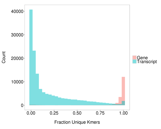
Figure 1. Distribution of unique sequence for genes and transcripts. The fraction of unique kmers (31mers) represents the “uniqueness” of the transcript. For transcripts, each kmer is classified as unique to that transcript or non-unique. For genes, a kmer is considered unique if it is only observed in transcripts of from a single gene. Genes are more unique than transcripts.

The biological question in hand will obviously largely dictate whether transcript-level quantification is required, but other factors are also important, including the accuracy of the resultant quantification and the availability of tools for downstream analyses. For my part, I’ve tended to focus on gene-level quantification unless there is a specific reason to consider individual transcripts, such as splicing factor mutation which will specifically impact expression of particular isoforms rather than genes as a whole. I think this is probably a common view in the field. In addition, every RNA-Seq dataset I’ve worked with has always been generated for the purposes of discovering differentially expressed genes/transcripts between particular conditions or cohorts. A considerable amount of effort has been made to decide how to best model read count gene expression data and, as such, differential expression analysis with read count data is a mature field with well supported R packages such as DESeq2 and EdgeR. In contrast, differential expression using isoform abundance quantification is somewhat of a work in progress. Of course, it’s always possible to derive gene-level quantification by simply aggregating the expression from all transcripts for each gene. However, until recently, transcript-level quantification tools did not return estimated transcript counts but rather some form of normalised expression such as fragments per kilobase per million reads (FPKM). Thus, to obtain gene-level counts for DESeq2/edgeR analysis, one needed to either count reads per gene or count reads per transcript and then aggregate. Transcript-level gene counting is not a simple task as when a read counting tool encounters a read which could derive from multiple transcripts it has to either disregard the read entirely, assign it to a transcript at random, or assign it to all transcripts. However, when performing read counting at the gene level the tool only needs to ensure that all the transcripts a given read may originate from are from the same gene in order to assign the read to the gene . As such, my standard method for basic RNA-Seq differential expression analysis has been to first align to the reference genome and then count reads aligning to genes using featureCounts. Since the alignment-independent tools all return counts per transcript, it’s now possible to count reads per transcript and aggregate to gene-level counts for DESeq2/edgeR analysis. Note: This requires rounding the gene-level counts to the nearest integer which results in an insignificant loss of accuracy.

Simulation results

Given my current RNA-Seq analysis method and my desire to perform more accurate gene-level and transcript-level analysis, the primary questions I was interested in were:

1. How do the three alignment-free quanitifcation tools compare to each other for transcript-level and gene-level quantification?
2. For transcript-level quantification, how does alignment-independent quantification compare to alignment-dependent (cufflinks2)?
3. For gene-level quantification, how does alignment-dependent quantification compare to alignment-dependent (featureCounts)?

To test this, I simulated a random number of RNA-Seq reads from all annotated transcripts of human protein coding genes (hg38, Ensembl 82; see methods below for more detail) and repeated this 100 times to give me 100 simulated paired end RNA-Seq samples.

Quantification was performed using the alignment-independent tools directly from the fastq files, using the same set of annotated transcripts as the reference transcriptome. For the alignment-dependent methods, the alignment was performed with Hisat2 before quantification using Cufflinks2 (transcripts), featureCounts (genes) and an in-house read counting script, “gtf2table” (transcripts & genes). The major difference between featureCounts and gtf2table is how they deal with reads which could be assigned to multiple features (genes or transcripts). By default featureCounts ignores these reads whereas gtf2table counts the read for each feature.

In all cases, default or near-default settings were used (again, more detail in the methods). Transcript counts and TPM values from the alignment-independent tools were aggregated to gene counts. To maintain uniform units of expression, cufflinks2 transcript FPKMs and gtf2table transcript read counts were converted to transcript TPMs.

Gene-level results

A quick look at a single simulation indicated that the featureCounts method underestimates the abundance of genes with less than 90% unique sequence which is exactly what we’d expect as reads which could be assigned to multiple genes will be ignored. See Figure 2-5 for a comparison with salmon.

Figure 2. Correlation between ground truth and featureCounts estimates of read counts per gene for a single simulation. Each point represents a single gene. Point colour represents the fraction of unique kmers (see Figure 1).

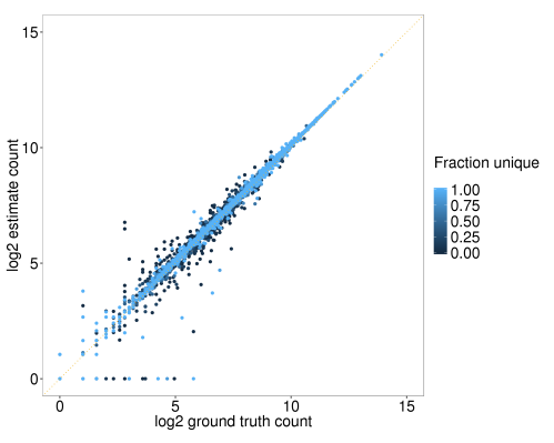
Figure 3. Correlation between ground truth and salmon estimates of read counts per gene for a single simulation. Each point represents a single gene. Point colour represents the fraction of unique kmers (see Figure 1).

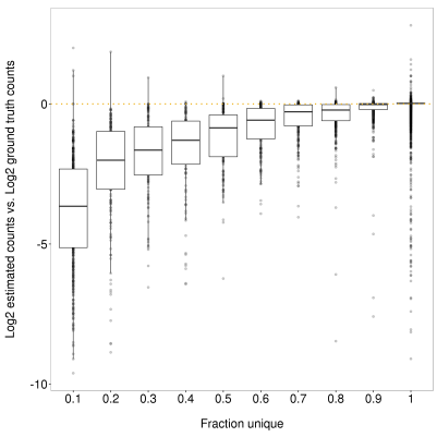
Figure 4. Impact of fraction unique sequence on featureCounts gene-level read count estimates. X-axis shows the upper end of the bin. Y-axis shows the difference between the log2 ground truth counts and log2 featureCounts estimate. A clear understimation of read counts is observed for genes with less unique sequence

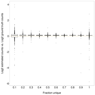
Figure 5. Impact of fraction unique sequence on salmon gene-level read count estimates. X-axis shows the upper end of the bin. Y-axis shows the difference between the log2 ground truth counts and log2 featureCounts estimate. Genes with less unique sequence are more likely to show a greater difference to the ground truth but in contrast to featureCounts (FIgure 4), there is no bias towards underestimation for genes with low unique sequence. The overall overestimation of counts is due to the additional pre-mRNA reads which were included in the simulation (see methods)

Since differential expression analyses are relative, the underestimation by featureCounts need not be a problem so long as it is consistent between samples as we might expect given the fraction of unique sequence for a given gene is obviously invariant. With this in mind, to assess the accuracy of quantification, I calculated the spearman’s rank correlation coefficient (Spearman’s rho) for each transcript or gene over the 100 simulations. Figure 6 shows the distribution of Spearman’s rho values across bins of genes by fraction unique sequence. As expected, the accuracy of all methods is highest for genes with a greater proportion of unique sequence. Strikingly, the alignment-independent methods outperform the alignment-dependent methods for genes with <80% unique sequence (11 % of genes). At the extreme end of the scale, for genes with 1-2% unique sequence, median spearman’s rho values for the alignment-independent methods are 0.93-0.94,  compared to 0.7-0.78 for the alignment-dependent methods. There was no consistent difference between featureCounts and gtf2table, however gtf2table tended to show a slightly higher correlation for more unique genes. There was no detectable difference between the three alignment-free method.

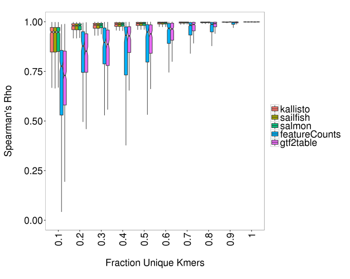
Figure 6. Spearman’s correlation Rho for genes binned by sequence uniqueness as represented by fraction unique kmers (31mers). Boxes show inter-quartile range (IQR), with median as black line. Notches represent confidence interval around median (+/- 1.57 x IQR/sqrt(n)). Whiskers represent +/- 1.5 * IQR from box. Alignment-independent tools are indistinguishable and more accurate than alignment-dependent workflows. featureCounts and gtf2table do not show consistent differences. All methods show higher accuracy with greater fraction unique sequence

 

Transcript-level results

Having established that alignment-independent methods are clearly superior for gene-level quantification, I repeated the analysis with the transcript-level quantification estimates. First of all,  I confirmed that the correlation between ground truth and expression estimates is much worse at the transcript-level than gene-level (Figure 7) as we would expect due to the aforementioned reduction in unique sequences when considering transcripts.

Figure 7. Correlation coefficient histogram for transcript-level and gene-level salmon quantification

Figure 8 shows the same boxplot representation as Figure 6 but for transcript-level qantification. This time only salmon is shown for the alignment-independent methods as kallisto and sailfish were again near identical to salmon. For the alignment-dependent methods, cufflinks2 and gtf2table are shown. Again, the alignment-independent methods are clearly more accurate for transcripts with <80% unique sequence (96% of transcripts), and more unique transcripts were more accurately quantified with alignment-independent tools or gtf2table. Oddly, cufflinks2 does not show a monotonic relationship between transcript uniqueness and quantification accuracy, although the most accurately quantified transcripts were those with 90-100% unique sequence. gtf2table is less accurate than cufflinks2 for transcripts with <15% unique sequence but as transcript uniqueness increases beyond 20%, gtf2table quickly begins to outperforms cufflinks2, with medium spearman’s rho >0.98 for transcripts with 70-80% unique sequence compared to 0.61 for cufflink2.

Figure 8. Spearman’s correlation Rho for transcripts binned by sequence uniqueness as represented by fraction unique kmers (31mers). Boxes show inter-quartile range (IQR), with median as black line. Notches represent confidence interval around median (+/- 1.57 x IQR/sqrt(n)). Whiskers represent +/- 1.5 * IQR from box. Alignment-independent tools are indistinguishable (only salmon shown) and more accurate than alignment-dependent workflows. gtf2table is more accurate than cufflinks for transcripts with >20% unique sequence. Alignment-independent methods and gtf2table show higher accuracy with greater fraction unique sequence. Cufflinks does not show a monotonic relationship between fraction unique kmers bin and median correlation coefficient.

The high accuracy of gtf2table for highly unique transcripts indicates that read counting is accurate for these transcripts. However, this method is far too simplistic to achieve accurate estimates for transcripts with less than 50% unique sequence (>86% of transcripts) for the reasons described above, and thus transcript read counting is not a sensible option for a complex transcriptome. The poor performance of cufflinks2 relative to the alignment-dependent method is not a surprise, not least because the alignment step introduces additional noise into the quantification from miss-aligned reads etc. However, the poor performance relative to simple read-counting suggests the inaccuracy is largely due to the underlying algorithm for estimating abundance which is less accurate than read-counting for transcripts with >15% unique sequence. This is really quite alarming if true (I’d be very happy if someone had any ideas where I might have gone wrong with the Cufflinks2 quantification?)

Overal conclusions and thoughts

As expected, accuracy was much higher where the transcript or gene contains a high proportion of unique sequence, and hence gene-level quantification is overall much more accurate. Unless one specifically requires transcript-level quantification, I would therefore always recommend using gene-level quantification.

From the simulations presented here, I’d go as far as saying there is no reason whatsoever to use read counting if you want gene counts and although I’ve not tested HTSeq, I have no reason to believe it should perform significantly better. From these simulations, it appears to be far better to use alignment-independent counting and aggregate to the gene level. Indeed, a recent paper by Soneson et al  recommends exactly this.

Even more definitively,  I see no reason not to use alignment-dependent methods to obtain transcript-level quantification estimates since the alignment-independent are considerably more accurate in the simulations here. Of course, these tools rely upon having a reference transcriptome to work with which may require prior alignment to a reference genome where annotation is poor. However, once a suitable reference transcriptome has been obtained using cufflinks2, bayesassembler, trinity etc, it makes much more sense to switch to an alignment-independent method for the final quantification.

In addition to the higher accuracy for the point expression estimates, the alignment-independent tools also allow the user to bootstrap the expression estimates to get an estimate of the technical variability associated with the point estimate. As demonstrated in the sleuth package, the bootstraps can be integrated into the differential expression to partition variance into technical and biological variance.

The alignment-independent methods are very simple to integrate into existing workflows and run rapidly with a single thread and minimal memory requirements so there really is no barrier to their usage in place of read counting tools. I didn’t observe any significant difference between kallisto, salmon and sailfish so if you’re using just the one, you can feel confident sticking with it! Personally, I’ve completely stopped using featureCounts and use salmon for all my RNA-Seq analyses now.

[EDIT] : Following the comment from Ian Sudbery I decided to have a look at the accuracy of expression for transcripts which aren’t expressed(!)

Quantification accuracy for unexpressed transcripts

Ian Sudbery comments below that he’s observed abundant non-zero expression estimates with kallisto when quantifying against novel transcripts which he didn’t believe were real and should therefore have zero expression. The thrust of Ian’s comment was that this might indicate that alignment-dependent quantification might be more accurate when using de-novo transcript assemblies. This also lead me to wonder whether kallisto is just worse at correctly quantifying expression of unexpressed transcripts which causes problems when using incorrectly assembled transcript models? So I thought I would use the simulations to assess the “bleed-through” of expression from truly expressed transcripts to unexpressed transcripts from the same gene – something that CGAT’s technical director Andreas Heger has also mentioned before. To test this I re-ran the RNA-Seq sample simulations but this time reads were only generated for 5592/19947 (28%) of the transcripts included in the reference genome; 78% of the transcripts were truly unexpressed. The figure below shows the average expression estimate over the 100 simulations for the 14354 transcripts from which zero reads were simulated (“Absent”) and the 5592 “Present” transcripts. Ideally, all the abscent transcripts should have expression values of zero or close to zero. Where the expression is above zero, the implication is that the isoform deconvolution/expression estimation step has essentially miss-assigned expression from an expression transcript to an unexpressed transcripts. There are a number of observations from the figure. The first is that some absent transcripts can show expression values on the same order of magnitude to the present transcripts, regardless of the quantification tool used, although the vast majority do show zero or near-zero expression. Within the three alignment-independent tools, kallisto and sailfish are notably more likely to assign truly unexpressed transcripts non-zero expression estimates, compared to salmon, even when the transcript sequence contains a high proportion of unique kmers. On the other hand, cufflinks2 performs very poorly for transcripts with little unique sequence but similarly to salmon as the uniqueness of the transcript increases. This clearly deserves some further investigation in a separate post…

Average expression estimates for transcripts which are known to be absent or present in the simulation. Fraction unique kmers (31-mers) is used to classify the “uniqueness” of the transcript sequence. Note that cufflinks2 systematically underestimates the expression of many transcripts, partly due to overestimation of the expression of “absent” transcripts.

Caveats

The simulated RNA-Seq reads included random errors to simulate sequencing errors and reads were simulated from pre-mRNA at 1% of the depth of the respective mRNA to simulate the presence of immature transcripts. No attempt was made to simulate biases such as library preparation fragmentation bias, random hexmer priming bias, three-prime bias or biases from sequencing. This purpose of this simulation was to compare the best possible accuracy achievable for each workflow under near-perfect conditions without going down the rabbit hole of correctlysimulating these biases.

[EDIT: The original text sounded like a get-out for my bolder statements ] Some comparisons may not be considered “fair” given that the alignment-free methods only quantify against the reference transcriptome where as the genome alignment-based methods of course depend on alignment to the reference genome and hence can also be used to quantify novel transcripts. However, the intention of these comparisons was to provide myself and other potential users of these tools with a comparison between common workflows to obtain expression estimates for differential expression analysis, rather than directly testing e.g kallisto vs. Cufflinks2.

The intention of this simulation is to provide myself and other interested parties with a comparison of alignment-independent and dependent methods for gene and transcript level quantification. It is not intended to be a direct comparison between featureCounts and Cufflinks2 and salmon, sailfish and kallisto – a direct comparison is not possible due to the intermediate alignment step – it is a comparison of the alignment-dependent and independent workflows for quantification prior to differential expression analysis when a reference transcriptome is available.

 

If you really want some more detail…

Methods

Genome annotations

Genome build:hg38. Gene annotations = Ensembl 82. The “gene_biotype” field of the ensembl gtf was used to filter transcripts to retain those deriving from protein coding genes. Note, some transcripts from protein coding genes will not themselves be protein coding. In total, 1433548 transcripts from 19766 genes were retained

Unique kmer counting

To count unique kmers per transcript/gene, I wrote a script available through the CGAT code collection, fasta2unique_kmers. This script first parses through all transcript sequences and classifies each kmer as “unique” or “non-unique” depending on whether it is observed in just one transcript or more than one transcript. The transcript sequences are then re-parsed to count the unique and non-unique kmers per transcript. To perform the kmer counting at the gene-level, kmers are classified as “unique” or “non-unique” depending on whether it they are observed in just one gene (but possibly multiple transcripts) or more than one gene. kmer size was set as 31.

Simulations

I’m not aware of a gold-standard tool for simulating RNA-Seq data. I’ve therefore been using my own script from the CGAT code collection (fasta2fastq.py). For each transcript, sufficient reads to make 0-20 copies of each transcripts were generated. Paired reads were simulated at random from across the transcript with a mean insert size of 100 and standard deviation of 25. Naive sequencing errors were then simulated by randomly changing 1/1000 bases. In addition reads were simulated from the immature pre-mRNA at a uniform depth of 1% of the mature mRNA. No attempt was made to simulate biases such as library preparation fragmentation bias and random hexmer priming bias or biases from sequencing since the purpose of this simulation was to compare the best possible accuracy achievable for each workflow under near-perfect conditions.

Alignment-independent quantification

Kallisto (v0.43.0), Salmon (v0.6.0) and Sailfish (v0.9.0) were used with default settings except that the strandedness was specified as –fr-stranded,  ISF and ISF respectively. Salmon index type was fmd. kmer size was set as 31.

Simulations and alignment-independent quantification were performed using the CGAT pipeline pipeline_transcriptdiffexpression using the target “simulation”.

Read alignment

Reads were aligned to the reference genome (hg38 ) using hisat2 (v2.0.4) with default settings except –rna-strandness=FR and the filtered reference junctions were supplied with –known-splicesite-infile.

Alignment-dependent quantification

featureCounts (v1.4.6) was run with default settings except -Q 10 (MAPQ >=10) and strandedness specified using -s 2. Cufflinks2 was run with default setting with the following additional options, –compatible-hits-norm –no-effective-length-correction. Removing these cufflinks2 options had no impact on the final results.