Estimating the number of true cell barcodes in single cell RNA-Seq (part 2)

This post starts where we left off in the first part. If you haven’t already done so, I’d recommend reading the first part now.

I hadn’t planned on writing another post but no sooner had I finished the first part of this blog post than I discovered that the Pachter group have developed a tool to perform the same task (sircel, pronounced ‘circle’). This appears to be in the early stages of development but there’s a bioAxiv manuscript out which happens to cover the same input data as I discussed in the previous post (thanks to Avi Srivastava for bringing this to my attention).

In the discussion with Avi in the comments of the previous post I also realised that I had failed to clarify that only base substitutions will be detectable when using our network methods. As it happens, one of the motivations for the development of sircel appears to be handling INDELs which they claim can be present in >25% of dropseq barcodes. I can’t see where they get this number from (In the manuscript they reference the original Macosko et al paper but I can’t see this 25% figure anywhere) so I’m assuming for now that this is based on additional analyses they’ve performed. This seems like an alarmingly high figure to me given that the rate of INDELs is ~1 order of magnitude less frequent than substituions (see Fig. 2/Table 2 here) and even at the start of the read where the cell barcode resides, the per-base rate of INDELs does not usually exceed 0.001. I would also assume that cell barcodes with INDELs would have far fewer reads and so drop below the threshold using the ‘knee’ method. Hence, while some cell barcodes may be discarded due to INDELs, I would be surprised if a INDEL-containing barcode was erroneously included in the accepted cell barcodes.

How common are INDELs?

Before I tested out sircel, I wanted to independently assess what proportion of cell barcodes might have a substitution or INDEL. To do this, I returned to the drop-seq data from the last post (GSE66693). Previously, I showed the distribution of reads per cell barcode separated into 4 bins, where bin 4 represents the accepted barcodes above the knee threshold and bins 1-3 are largely populated by different types of erroneous barcodes (reproduced below as Figure 1). I compared each barcode to all barcodes in bin 4 and looked for a match allowing for one error (substitution, insertion or deletion). The results are tabulated below.  These figures are an upper estimate of the number of barcodes/reads harbouring an error relative to the true cell barcodes since each barcode may contribute to all three error types if at least one match to a bin 4 barcode exists with each error type. We can see that ~1.5% of cell barcodes may contain an INDEL, far less than the 25% suggested in the sircel manuscript. Furthermore, when we present the figures according to the number of reads, it appears around 3% of reads have a cell barcode with an INDEL, whilst 7% have a substitution. Thus, we can be quite confident that we’re not losing lots of data if we don’t error correct cell barcodes or just correct substitution errors.

indrop_bins

Figure 1. Distribution of reads per cell barcode (log 10) from first 50M reads, separated into 4 bins. Bin 4 represents the ‘true’ barcodes.

Untitled 2

Table 1: Columns 1 & 2: The number and fraction of cell barcodes which match a bin 4 barcode allowing one error. Columns 3 & 4: The number and fraction of reads with a cell barcodes which match a bin 4 barcode allowing one error.

Are INDEL-containing barcodes passing the knee threshold?

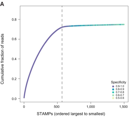
Next, I want to investigate whether the INDEL barcodes pass the knee threshold and become ‘accepted’. I therefore split the above data according to bin and focused on bin 4. As you can see in Figure 2 below,  there are indeed a small number of bin 4 barcodes which are a single error away from another bin 4 barcodes. Our null expectations (from 100 000 randomly generated barcodes) for the percentage of subsitution, deletion and insertion matches by chance are 0.14, 0.11 and 0.13%, respectively. In contrast, amongst the 575 bin 4 barcodes, there are 6 barcodes (1.0%) which match at least one other bin 4 barcode with one error. 4/6 of these barcodes have a match with an INDEL and all have relatively low counts suggesting these are indeed errors. It seems I may have been wrong to assume a INDEL-containing barcodes will not pass the knee threshold. The results for bins 1-3 minor my previous analysis using edit-distance and suggest the bin3 is mainly made up of error-containing barcodes whilst bins 1 & 2 appear to originate from amplification of ambient RNA in empty droplets.

error_detectionFigure 2. The frequency of cell barcodes in each bin which are one error away from at least one of the bin 4 barcodes. Random = 100 000 randomly generated barcodes

How does sircle compare to the knee method?

So, INDELs are observed in this drop-Seq data, although perhaps not 25% of all cell barcodes, and INDEL-containing barcodes can pass the hard knee threshold for acceptance. Now on to sircel. As you would expect from the Pachter group, sircel introduces a novel, elegant solution to detect substitutions and INDELs in barcodes. Rather than using edit-distance or fuzzy matching, they ‘circularise’ the barcodes and form a de Bruijn graph using the kmers from the circularised barcodes. The circularisation ensures that even with a large kmer size, barcodes containing an error will share at least a portion of their path through the de Bruijn graph with the cognate error-free barcodes. The edges are weighted according to the number of times each edge is observed and each circular path is given a score according to the minimal weight of all its edges. This score is used to filter the paths to select the high weight, correct paths and incorrect paths are merged to the correct paths. Notably, the thresholding is done using a method analogous to the knee method, whereby the threshold is set as the local maxima of the smoothed first derivative from the cumulative distribution of path scores. The neat thing about the sircel method is that it enables simultaneous identification of this inflection point to identify the threshold for true barcodes, and error correction to the true barcodes. To compare the results for sircel and my knee method, I ran sircel on the GSE66693 drop-seq sample where the authors had suggested there were ~570 true cell barcodes. Previously, using the first 50M reads I had estimated that there were 573 true barcodes using the knee method. As per the sircel manuscript recommendation, I used only 1M reads to run sircel, which yielded 567 true barcodes. This is slightly lower than the number quoted in the manuscript for 1M reads (582) but perhaps this is due to more recent updates? The methods agree on 563 cell barcodes but what about the cell barcodes where they agree. 4/10 out of the knee method-specific cell barcodes are a single error away from another barcode above the threshold, suggesting these may in fact be errors. The remaining 6 barcodes all have very low counts. Likewise, the 4 sircel-specific cell barcodes fall just below the knee threshold (6170-9576 reads per barcode; threshold = 9960). For these 10 barcodes, the difference appears to be due to differences in the number of reads sampled. I wanted to check this by using 50M reads with sircel but the run-time becomes excessively long. Unfortunately, going to other way and using just 1M reads with the knee method yields unstable estimates and since it takes <6 minutes to run the knee method with 50M reads we would never recommend using the knee method with just 1M reads. So in essence, the major difference between the knee method and sircel is that sircel effectively corrects the small number of error barcodes above the threshold.

Can we improve the knee method?

It does look like sircel does a good job of removing error barcodes but we could easily replicate this performance by performing an INDEL-aware error detection step after the knee threshold. During the development of UMI-tools we considered detecting INDELs as well as substitutions but decided against it because: a) as mentioned at the top, the rate of INDELs is usually ~1 order of magnitude lower than substituions (that this doesn’t appear to hold true for cell barcodes), and b) UMI-tools groups reads together by their alignment position so the current framework does not allow the detection of INDELs. However, when we’re dealing with cell barcodes, we consider all barcodes at once and hence, it’s much easier to identify INDELs. For our network methods, we can simply replace the edit-distance threshold with a fuzzy regex, allowing one error (substitution, insertion or deletion). The fuzzy regex matching is ~30-fold slower than our cythonised edit-distance function but this isn’t an issue here since we only need to build the network from the cell barcodes which pass the knee threshold. From the network we can identify the error barcodes and either correct these to the correct barcode or else discard them. This will now be the default method for UMI-tools extract with the option to discard, correct or ignore potential barcode errors above the knee threshold. We will also include the option to correct barcodes which fall below the threshold.

A final thought: To correct or not?

The cost of incorrectly merging two cell barcodes through cell barcode error correction could be drastic, e.g appearing to create cells ‘transitioning’ between discrete states. On the other hand, discarding reads from error barcodes rather than correcting them reduces the sequencing depth and hence increases the noise. In the drop-seq data above 55.7% of reads are retained without error correction with a further 9.2% of reads potentially correctable. If all barcodes above the threshold and within one error of another barcode above the threshold were removed, this would only mean the loss of 0.3% of reads. Given the potential dangers of incorrect error correction, it may be prudent in some cases to discard all cell barcodes with errors and work with 55.4% of the input reads rather than correcting errors in order to retain 64.9% or reads

Estimating the number of true cell barcodes in single cell RNA-Seq (part 1)

Single Cell RNA-Seq (scRNA-Seq) took a major leap forward in 2015 when two Harvard groups published oil droplet-based methods for sequencing >10,000 cells in a single experiment for << 1$ / cell (Klein et alMacosko et al). Then in early 2016, 10X Genomics launched their commerical version of droplet scRNA-Seq, followed more recently by the illumina and Bio-Rad competitor technology. From my limited exposure, the 10X product seems to be the most popular right now but this is a very new field so there are likely more improved methods on the horizon which could shake things up. These techniques label cells in fundamentally in the same manner. Using microfluidic devices individual cells are encapsulated together with a random cell barcode in a droplet. The reverse transcription of the RNA and subsequent PCR amplification is then performed inside each droplet separately such that all cDNA from a single cell are labelled with the same cell barcode.

The techniques themselves are really exciting but I want to focus here on a technical question during the analysis. A crucial aspect of droplet scRNA-seq is that the number of possible cell barcodes is many orders of magnitude greater than the number of cells sequenced. Hence, if each sequenced cell gets one cell barcode at random, the probability of two cells having the same barcode is very low (if you’re interested, you can work out the probability using the solution to the famous ‘birthday problem’). However, when you get your sequencing data back and extract the cell barcodes detected, not all of these will be ‘true’ cell barcodes and some barcodes will contain sequencing errors or PCR errors. Furthermore, some cell barcodes may have been incorporated into cDNA that does not originate from your cells (more on this later). Hence, one of the first challenges in droplet scRNA-Seq is working out how many cells you’ve actually sequenced! In the supplementary material of the original drop-seq paper (Macosko et al) they suggest plotting the cumulative frequency and looking for an inflection point, or ‘knee’. They show this in supplementary Figure 3A (reproduced below in Figure 1 with permission). The 10X analysis pipeline also appears to take a similar approach by what I can gather from their website.

figs3_lrg-e1495127255597.jpg

Figure 1. Cumulative frequency for drop-seq data. Plot taken from Macosko et al supplementary figure 3 with permission.  Dashed line shows inferred position of point of inflection.

Now, if you’ve been on this blog before, you’ll probably have seen the posts about UMI-tools. This is a tool suite I’ve co-developed with Ian Sudbery (University of Sheffield) to accurately identify PCR duplicates in techniques utilising unique molecular identifiers (UMIs). UMIs are similar to cell barcodes in that they are just a sequence of bases used to barcode a read, though in this case, the barcode relates to the unique molecule prior to PCR amplification. The novel aspect of our tools is that we used networks to identify PCR duplicates in an error-aware manner. For background on the network methods, please see our publication or my previous blog post.  For the next major UMI-tools release (version 0.5), we’re planning to expand our support for single cell RNA-Seq analyses as this seems to be the major application of the tool to date according to our GitHub issues. As part of this, we wanted to expand the extract command. Currently this command extracts the UMI sequence from the reads and appends it to the read name so that the UMI can be accessed in the downstream BAM, We wanted to extend the extract command so that it can

  • extract cell barcodes
  • filtered cell barcodes against a whitelist of expected cell barcodes
  • or, where no whitelist exists (as in the case of droplet scRNA-Seq), create a whitelist of ‘true’ cell barcodes from the data and filter against this

For the final point, we needed to implement an automated version of the ‘knee’ method as described in the drop-seq paper. We also wondered whether our network based methods might be suitable for this purpose as they are designed to handle the situation where you have an unknown number of ‘true’ barcodes plus additional barcodes which have been generated via errors from the ‘true’ barcodes. I therefore set out to implement a ‘knee’ method and compare it with our network methods.

To start with, I took the SCRB-Seq data from Soumillon et al since I had it to hand and this includes 384 expected cell barcodes which I could use as a ground truth. All other barcodes observed should therefore have originated as errors from the 384 true barcodes. To be clear, this is not droplet scRNA-Seq but this give us a definitive ground truth for the purposes of initiation performance testing. Plotting the cumulative frequency we can clearly see an inflection near the 384th barcode as expected (Figure 2; blue line).

no_methods_cumsum

Figure 2. Cumulative frequency for SCRB-Seq cell barcodes. Blue line represents the position of the 384th cell which is close to the inflection point in the curve.

I initially attempted to identify the inflection point by fitting a spline function to the cumulative frequency but quickly realised it was much easier to work from the distribution of counts (log10) per cell barcode (Figure 3). Here the inflection point is represented by the local minima between the distribution of counts for ‘true’ and ‘false’ barcodes. We can see that the local minima is very close to the 384th cell barcode so this automated knee method seems to work well for this data. The obvious downside of this hard thresholding on read counts with the knee method is that there will likely be some overlap between the read counts for real and false barcodes (as we can see in Figure 3) . This is why we believed the network-based methods may be more accurate.

scrb_seq_one_min_dist

Figure 3. Density of reads per SCRB-Seq cell barcode. Blue line represents the position of the 384th cell which is close to the inflection point in the curve in figure 2. Orange line represents the local minima used in my implementation of the ‘knee’ method.

To compare with our network-based methods, I took increasing samples of reads from the SCRB-Seq sample and estimated the true cell barcodes using the knee method and our ‘adjacency’ and ‘directional’ methods and calculated the sensitivity and false positive rate (FPR) of the different approaches. As you can see in Figure 4, the ‘directional’ method has a slightly higher sensitivity and lower FPR than the ‘knee’ method, which suggests that this network-based method might be more suitable for identifying the true cell barcodes. The knee method slightly outperforms just selecting the top 384 most abundant barcodes (‘top 384’) in terms of higher sensitivity although this comes at the cost of increased FPR. The ‘adjacency’ method has a high sensitivity but tends towards overestimating the number of true cell barcodes as the number of sampled reads is increased. This is because adjacency only groups barcodes together if they are all separated from the same hub barcode and each by a single edge. Hence, any barcode with 2 or more errors will be always be in a separate group from the true barcode from which it originates. In contrast, the directional method is not limited to single edge paths.

pSens_zoom.pngpFPRpFPR_zoom

Figure 4. Sensitivity (Top) and False Positive Rate (FPR; Middle, Bottom) for 3 methods to detect the number of true cells sequenced. “Top 384” = select the top 384 barcodes. Shown for comparison with knee method. Middle = all samples. Bottom = adjacency excluded to show difference between knee and directional.

Next, I took a single sample from the drop-seq paper where the authors had inferred that there were ~570 cells using a visual assessment of the cumulative frequency plot (This is the sample shown in Figure 1). They also backed up this assertion with an assessment of the species-specificity of the reads for each cell barcode which suggested that most of the “cells” below this inflection point were actually droplets which did not contain a cell and simply contained ‘ambient’ RNA. So, 570 seemed a reasonable truth to test the method against. My ‘knee’ method worked great, using the first 50M reads, this method estimated that there were 573 cell barcodes (Figure 5).

indrop_cumsum

Figure 5. Cumulative frequency plot for cell barcodes in the first 50M drop-seq reads. The ‘knee’ method estimated 573 true cell barcodes and hence is plotted over the ‘top 570’ inflection point prediction. The X-axis has been limited to the 10 000 most abundant cell barcodes.

In contrast, the directional method failed miserably! For starters, the shear number of cell barcodes precluded the inclusion of all cell barcodes detected as the network building requires an all-vs-all comparison between the barcodes to calculate the edit distances. With 50M reads, the sensitivity was OK (95%), but the specificity was just 11% and the specificity unexpectedly increased as the number of reads parsed was decreased! Then came the realisation…

Image result for homer doh

As mentioned above, the network-based methods were designed to deal with a pool of barcodes, where some barcodes are true and the remaining barcodes are the result of errors from the true barcodes. However, here we have a situation where the ‘false’ barcodes could be due to either errors (I’ll call these ‘error barcodes’), or droplets without a cell which have amplified ambient RNA (‘ambient barcodes’). We can indentify these two separate types of false barcodes by looking at the minimum edit-distance between each barcode and the true barcodes. For error barcodes, we would expect this minimum edit-distance to be 1 in most cases. For ambient barcodes we expect them to have a similar distribution of minimum edit distances relative to the true barcodes as barcodes selected at random. Figure 6 below shows the distribution of counts per barcode, split into 4 bins. Figure 7 shows the distribution of edit-distances for each bin and a null distribution from a randomly generated set of cell barcodes. Bin 4 contains the true barcodes and shows a null-like distribution of edit-distances as expected. We can clearly see that bin 3, which has slightly lower counts per cell barcode compared to the true barcodes, is enriched in single edit-distances relative to the null. This strongly suggests many of these cell barcodes are error barcodes with a single error relative to the true cell barcode from which they originate. However, bin 2, and bin 1 especially, show a more null-like distribution, suggesting most of these cell barcodes are instead ambient barcodes.

indrop_bins

Figure 6. Distribution of reads per cell barcode (log 10) from first 50M reads, separated into 4 bins. Bin 4 represents the ‘true’ barcodes.

edit_distances_drop_seq

Figure 7. Distribution of minimum edit distance compared to true barcodes (bin 4) for each bin shown in figure 6. Random = 10 000 randomly generated cell barcodes.


In summary, the knee method as implemented here works very well with the samples tested so far so we can proceed with automatic detection of the number of true cell barcodes with UMI-tools extract. We will also enable the use of the directional method since this is more accurate when you know that all false cell barcodes are the result of errors. However, I’d recommend sticking with the knee method unless you are absolutely certain this is the case.

Finally, if you’re already using UMI-tools for scRNA-Seq, or thinking about doing so, keep a look out for version 0.5. Along with the added functionality discribed here, we’re adding a count commands to yield counts per cell per gene directly from featureCounts/HTSeq output and we hope to include a scRNA-Seq-specific tutorial for this release too.

EDIT: Following the comments below I’ve continued this analysis into a second post to look at INDELs in cell barcodes and comparing UMI-tools with sircel.

The dependency hell in software development

Introduction

Most software projects depend on other software packages to provide its functionality. Actually, the bigger your software project, the more likely is that you end up having a large number of dependencies either internally between different parts of your code or externally with third-party libraries.

The goal of adding a new dependency to your code is to avoid reinventing the wheel. If there is code already available that does what you want, normally you would prefer to re-use it (there are exceptions, though) rather than investing your time in re-writing new code to solve the same task. On the other hand, once your software project has matured over time and is ready for production it may end up being a dependency for other software projects as well.

Grouping off-the-shelf functions into software packages and defining dependencies between them has been traditionally at the core of software development. It is specially important if you try to follow the Unix Design Philosophy where the aim is to build small programs that do one thing well, and can be easily re-used.

At the time that you decide to write new software to solve a problem that is not being tackled by other software out there, you will also have to choose the operating system, the programming language, system libraries, and a collection of other software packages available on the system. These choices will create dependencies between your new piece of code and a specific software environment that will need to be reproduced to run properly on a different system.

Initially, re-using software packages as much as possible looks like the best way forward to save time and effort in the long run; and it is indeed true. However, creating dependencies with other software packages also brings its own disadvantages, specially when the number of dependencies becomes larger and larger. Here is a nice example illustrating what I am talking about.

gentoo-deps

Copy and paste the original text to explain the picture:

This graph shows the dependencies between software packages in the Gentoo Linux operating system. In total there are 14,319 packages with 63,988 dependencies between them!

Packages are drawn on the circumference of the circle and a dependency is indicated by a line draw from one package to another. The colour of a package is randomly generated, while the colour of a line is determined by the package that is required by the other packages.

Every package has a line starting on the rim of the circle drawn radially outwards. The length of the line is determined by the amount of other packages that depend on the package.

As you can imagine, the larger the number of dependencies between packages, the more likely is to create conflicts between them (among other issues). This problem is known as the dependency hell and is the driver for the rise of new technologies out there, like containers, that are trying to propose a feasible solution.

The example about Gentoo Linux might seem an extreme one. However, the codebase in CGAT currently depends on 58 R packages and 45 Python packages, plus third party tools available in our compute cluster, where we have over 200 packages installed. Click here if you dare to check out the graph of internal dependencies for the CGAT scripts!

In the rest of this post I will revisit quickly how the dependency hell problem has been addressed up to date, from no dependency resolution at all to the full isolation provided by containers. Then, I present how I have approached the dependency hell problem for the CGAT scripts. Finally, I provide my conclusions and some advice that will hopefully be useful for someone out there.

A brief history of open-source software distribution

Before talking a bit more about containers, let us now have a quick look at the evolution of how open-source software has been distributed since the Internet was available.

Tarballs

Back in the old days the only way of sharing software was to create a tarball containing the code, configuration files and scripts to compile/install the code. As mentioned, unless the software package was completely self-contained, the dependencies were not shipped with it and if you did not have them installed on your box, it would rapidly complain either at compilation or run time. The amount of time spent making the new software package to run properly varied with the number of dependencies and the conflicts with the packages already installed. Finding the right versions for all the dependencies manually was a big limitation preventing the distribution of open source software, if not impossible in some cases.

Another problem was to build the software package on a CPU architecture that was compatible with the target system. Nowadays, the amount of different CPU architectures available in the market has shrunk quite a lot, but that has not been always the case.

Having said that, it is also true that if your software only depends on a couple of packages, and your reference CPU architecture is the widely used x86, tarballs are still today a feasible way of sharing code (although you should consider better options as explained below!)

Package managers

In order to ease the distribution of open source software, package managers were created. Instead of sharing just the code, the software was pre-compiled in a reference CPU architecture and packaged into special file format that included a way of specifying where the code should be located in the destination file system along with a list of the required software dependencies and version numbers. RPM and APT are probably the most popular package managers for Red Hat and Debian based Linux distributions, respectively.

Depending on the complexity of a software project, it is not trivial to create a package for a package manager. However, the benefits are evident. The package just needs to be uploaded to a proper repository and it can be easily installed by end users with no effort via the package manager, which will download the package and all its dependencies if they are not installed on the target system.

Although dependency resolution is a key feature of a package manager, it is worth mentioning that advanced package managers also play other important roles like applying security updates in a timely manner or checking that the software to be installed is not malicious.

Package managers started as a core part of Linux distributions but the list has grown to other operating systems as well. The concept has been extended outside operating systems to manage packages for programming languages like Perl, Python and R to name a few. Even more remarkable are initiatives like Conda, a package manager that was initially intended for Python packages only but has been generalised to manage packages in different programming languages (Python, R, Ruby, Lua, Scala, Java, Javascript, C/ C++ and FORTRAN) and can be installed in all the major operating systems in the market (Linux, OS X and Windows). More about Conda later.

Virtual machines

When the number of dependencies either with other software packages or with the underlying operating system is quite specific and/or large, another approach is to create a virtual machine where the complete software stack is under control. Virtual machines can be shared via its virtual disk only or as virtual appliances. The former gives freedom to the end user to select the amount of virtual resources assigned to the virtual machine (e.g. number of CPU cores and size of main memory). The latter not only comes with the software pre-installed but also with the virtual resources pre-selected for you so your hypervisor of choice just runs it.

Containers

Since Docker irrupted in 2014, there has been a lot of hype around containers in software development in the last years. Here is a good definition of containers:

Using containers, everything required to make a piece of software run is packaged into isolated containers. Unlike virtual machines, containers do not bundle a full operating system – only libraries and settings required to make the software work are needed. This makes for efficient, lightweight, self-contained systems and guarantees that software will always run the same, regardless of where it’s deployed.

Docker is available for all major operating systems (Linux, OS X and Windows) and the idea is that you create a container for your application once, and it runs everywhere. That is quite appealing and is the reason why Docker in particular, and containers in general, are getting a huge attention these days.

Conda package for CGAT scripts

CGAT maintains a collection of scripts and pipelines for the analysis of high-throughput sequencing data. As stated above, the code has a large number of dependencies and it has been traditionally a challenge to deploy outside the CGAT cluster. Basically, we are facing the dependency hell ourselves and here I describe our approach to solve it.

In the past, I have been playing more or less with several options presented in this post to make our code portable. Right now, I consider Conda the most suitable option going forward but time will tell whether I am wrong or not.

Conda is easy to learn and install plus there are already a couple of community led efforts that make this option attractive: Bioconda and conda-forge. These teams are making great contributions to enable reproducible research and solve the dependency hell problem. Special thanks to Johannes Köster for setting out the Bioconda community and asking me to become a contributor. I am also grateful to Bioconda’s the core team for their hard work and dedication to keep this project moving on.

Recently, I have added a Conda package to the Bioconda channel for the CGAT scripts. Next, I will describe the installation steps so you can give it a try and confirm whether the Conda approach is really a solution to our dependency hell!

The installation instructions below are for Linux. OS X and Windows users must install Docker and use the container option. I will use the a temporary folder, but feel free to choose a different location on your system.

# create an installation folder
mkdir /tmp/conda
cd /tmp/conda

# download and install Conda
wget https://repo.continuum.io/miniconda/Miniconda3-latest-Linux-x86_64.sh
bash Miniconda3-latest-Linux-x86_64.sh -b -p /tmp/conda/install
export PATH=/tmp/conda/install/bin:$PATH

# configure Conda
conda config --set allow_softlinks False
conda config --add channels conda-forge
conda config --add channels defaults
conda config --add channels r
conda config --add channels bioconda

# install CGAT scripts into a Conda environment
conda create -n cgat-scripts cgat-scripts -y

Since the number of dependencies is high, the installation will take up to 10 minutes depending on your system’s configuration. According to my test, you’ll need 3GB of free disk space for the complete installation as well.

Now, you are ready to go:

# on the same or a different terminal, activate the Conda environment
source /tmp/conda/install/bin/activate cgat-scripts

# and now you should be able to use the CGAT scripts
cgat --help
cgat --help Genomics
cgat --help Conversion
cgat gtf2table -h
cgat bam2geneprofile -h

So all you need to decide is the path on your file system to install Conda and all the dependencies will be located under a single folder that you can then enable on demand. Please note, we have made use of Conda environments, which gives you flexibility to have a specific set of dependencies without conflicting with other environments (e.g. different versions of Python or R) on the same Conda installation. Or, if you are really paranoid about breaking things (like myself), you can create a separate Conda installation on a different location on your file system, to ensure full isolation.

If that worked for you, and are interested in more details about how the Conda package was created, please feel free to comment on this post and I will try to help.

Conclusions

In summary, I explained the dependency hell and how the problem has been tackled until today, and later I presented the Conda package for CGAT scripts as a way of solving our own dependency hell, which will hopefully work on your systems!

Finally, based on my experience solving the dependency hell for the CGAT scripts, here is my advice on how to address the problem properly if you are a software developer. Firstly, I recommend to be really picky when choosing new dependencies for your code. Make sure the software you depend on is in good health and maintained. Secondly, have a way of tracking the dependencies for your software. For example, a simple up to date list of software packages and the required versions will do the job.

matplotlib Tutorial

Hi Everyone,

I have made a quick tutorial on the basics of plotting with matplotlib.

It covers:

  • Matplotlib vocabulary – figures and axes
  • The different ways to use matplotlib: the interactive interface, the object-oriented interface and the object-oriented class library
  • Basic plotting commands
  • Customising plots using containers and artists

It is available to view here.

Or to download as an interactive IPython notebook here.

Good luck!

Katy